nserman@fsb.hr Transfer Function Concept Digest
12. RELATIONSHIP BETWEEN CLOSED-LOOP TRANSIENT DAMPING AND THE OPEN-LOOP FREQUENCY RESPONSE
Closed loop will be stable if the open-loop frequency response exerts positive stability margins. Stability margins ASM and PHSM are shown in Bode diagram in Fig. 11.1.
Their presentation in Nyquist diagram is shown in fig. 12.1. In Bode diagram ASM is expressed in dB while in Nyquist diagram it is a plain ratio of the amplitudes. They can be calculated from each other using relationships ![]() or
or ![]() .
.
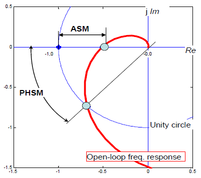
Figure 12.1 Amplitude and Phase Stability Margins in the Nyquist diagram coordinates
Closed loop is stable if the open-loop frequency response does not encircle point [ -1, j0 ]. By passing somewhere between the origin and point [ -1, j0 ] it exerts some ASM and PHSM, as shown in fig. 12.1. “Closed loop is stable” means that the transients converge to zero after a time. However, an existence of ASM and PHSM provides no information on the transients damping.
Such information can be reached by a family of αR = const circles, (where αR denotes resonant gain). It is sometimes referred to as Hall diagram. The coordinate of the resonant gain centers is defined as:
![]()
Each circle radius is:
![]()
Looking at it as a curves pure mathematical parametric description with 0 < αR < ∞ being a parameter, it presents a family of circles shown in fig. 12.2.
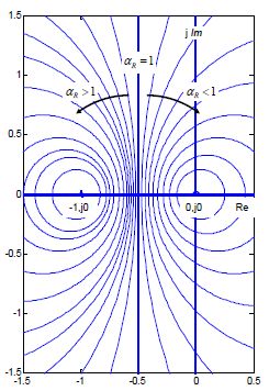
Figure 12.2 Family of αR = const circles in the region 0 < αR < ∞
In most control problems the closed-loop transfer function has one or more pairs of complex poles. Even in a case when closed loop is stable, the transients would most probably be oscillatory. That brings up a phenomenon of resonance. What we are interested in is the range of αR > 1. It means that the left-hand side of the plane in fig. 12.2 is what is relevant only, as is shown in fig. 12.3.
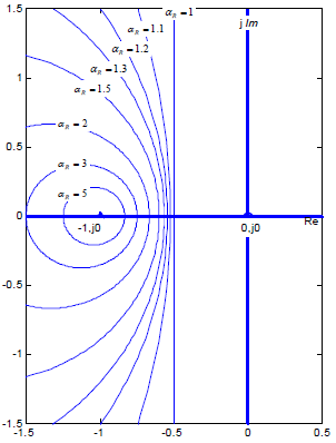
Figure 12.3 Closed loop αR = const circles in the open-loop Nyquist coordinates.
The second order oscillator is detailed in Chapter 10.6. The dynamics of a 2nd order stable system that is characterized by a single pair of complex poles has been presented there. The meaning of damping ratio and the resonance was explained as well. There is a relationship between resonant gain αR and damping ratio ζ :
![]()
There is also an expression for the opposite direction, expressing ζ as a function of αR :
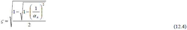
As per the above relationship unity resonance gain αR = 1 corresponds to the damping ratio ζ ≈ 0.7. That is considered as the optimal value for the closed-loop dynamics in most control applications. It offers the fastest transients fading without much risk of the resonance.
To get some idea about closed-loop transients damping there is a presentation in fig. 12.4. It shows the step responses for several characteristic values of damping ratio ζ and corresponding resonance gain αR .
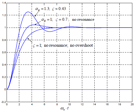
Figure 12.4 Step responses for several characteristic values of damping ratio ζ and corresponding resonance gain αR
Let us examine a hypothetical control loop whose open-loop frequency response in Nyquist diagram is presented by the red line in fig. 12.5. The open-loop frequency response does not encircle point [ -1, j0 ] and exerts positive stability margins ASM and PHSM. It means that the subject closed loop is stable.
Additionally it touches the circle αR = 1 .3. It would mean that the closed-loop transients will be damped at the damping ratio ζ ≈ 0.43 and would look as presented in fig. 12.4.
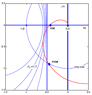
Figure 12.5 Open-loop frequency response of a hypothetical control loop (red line) in Nyquist diagram with ASM and PHSM points and αR = const circles
There is a question hanging at the end of this chapter: What could be a benefit of bothering with the open loop frequency response in Nyquist diagram when the information of the closed loop dynamics is obtainable?
The answer is simple. Due to the fact that the open loop structure is commonly characterized by a serial blocks connection, the influence of each blocks to the overall open loop frequency response is much more transparent than its influence to the closed loop behavior.