
nserman@fsb.hr Transfer Function Concept Digest
10. ELEMENTARY BLOCKS
10.2 Integrator
When the pole of the transfer function (10.2) equals zero, i.e. for p = 0, it presents the transfer function describing the elementary component commonly referred to as an integrator – fig 10.5
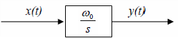
Fig. 10.5 Block presentation of an integrator
Remark
Integrator pole equals zero, i.e. p = ± 0 would actually jeopardize the assumption of all elementary blocks being stable. This assumption is relevant for the Nyquist stability criterion appropriate formulation in cases when there is one or more integrators within the open loop transfer function. Therefore, it is assumed that the complex plane origin belongs to the lefthand side of the plane, i.e. that it actually tends to zero from the negative side (simply symbolized by p = – 0). This remark is of no importance for applying the following content to engineering problems however, it is given here in order to preserve at least the minimal level of mathematical scrutiny.
In the time domain integrator is defined by the first-order differential equation (10.6)
![]()
after integration it becomes:
![]()
Transfer function of an integrator is:
![]()
where ω0 is a constant with dimension of angular frequency [rad/s] (therefore the symbol ω0).
Integrator behavior in the time domain is illustrated by its step response in fig. 10.6.
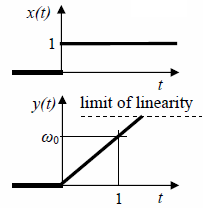
Fig 10.6 Integrator response to a unity step at the input, initial condition y(0) = 0.
Output y(t) is a straight line which goes to infinity. For real physical systems this infinity means the limit of linearity where the system still behaves as linear.
Frequency response of an integrator coincides with the negative part of the imaginary axis in Nyquist diagram, so φ = -90° regardless of the value of ω0, as is shown in fig. 10.7.
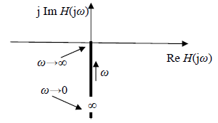
Fig 10.7 integrator frequency response in Nyquist diagram
Frequency response of an integrator in Bode diagram is shown in fig. 10.8. for three different values of ω0.
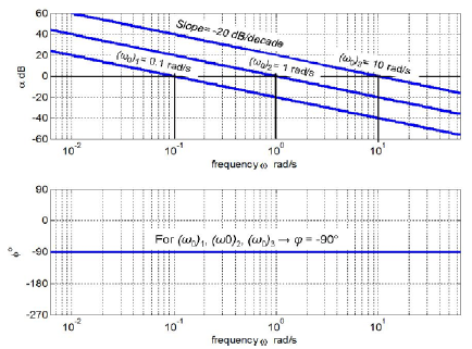
Fig 10.8 Frequency response of an integrator in Bode diagram for three different values of ω0.
Amplitude-frequency characteristic is a straight line with a slope of -20 dB/decade, which is referred to as negative unity slope (or slope = -1). Dynamic gain lines cross the unity gain axis (αdB = 0) at frequency ω0.
Phase-frequency characteristic is a horizontal straight line at φ = -90° regardless of the ω0 value.