
nserman@fsb.hr Transfer Function Concept Digest
10. ELEMENTARY BLOCKS
10.3 First Order Lag
When the pole of the transfer function (10.2) is a real negative number p = – ω0 and constant K equals ω0, the transfer function becomes:
![]()
In control engineering, this elementary block is named first-order lag or PT1. Its only parameter is referred to as time constant denoted by T , where ![]() . It is presented in fig. 10.9 in that form.
. It is presented in fig. 10.9 in that form.
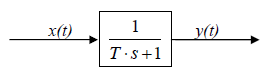
Fig 10.9 Block presentation of the first-order lag
First-order lag as an autonomous component is most often made by closing a negative unity feed-back around an integrator, as is shown in fig. 10.10.
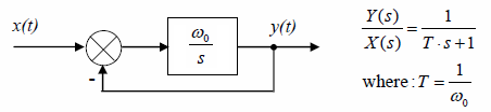
Fig 10.10 First-order lag internal structure
Relationship between the output y(t) and input x(t) in the time domain is defined by the equation:
![]()
First-order lag step response is shown in fig. 10.11.
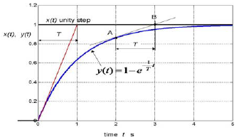
Fig 10.11 First order lag step response to unity step at the input (time constant T = 1s).
The step response provides an information on a shape of the monotonic summands in the complex system’s transients – chapter 5. The shape is defined by time constant T influence on the respective exponential function eσ0t with σ0 < 0, (for all the converging parts of the system transients). A time period between point A and point B is always equal T. Point A is any point where the tangent touches the curve. Point B is the point where the same tangent intersects the horizontal asymptote. Point A can be located anywhere at the curve itself.
Frequency response of a first-order lag in Nyquist diagram is presented in fig. 10.12. It is always a halve-circle with the unity diameter regardless of the time constant T value.
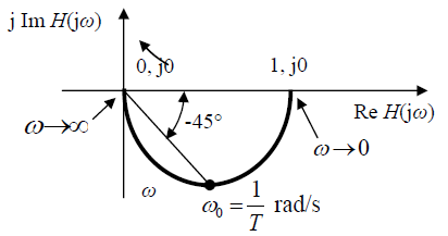
Fig 10.12 First-order lag frequency response in Nyquist diagram.
A first-order lag frequency response in Bode diagram is shown in fig. 10.13.
In a low frequency range, where ![]() , a first-order lag resembles the properties of static gain (αdB = 0, φ = 0°).
, a first-order lag resembles the properties of static gain (αdB = 0, φ = 0°).
In a high-frequency range, where ![]() , the characteristics coincide with their asymptotes that are resembling the properties of an integrator. The slope of the amplitude-frequency characteristic asymptote equals -20dB/decade, and the phase shift amounts -90° in the whole high-frequency range. Any variation in T would move the characteristics in the horizontal direction. Their shape always remains the same.
, the characteristics coincide with their asymptotes that are resembling the properties of an integrator. The slope of the amplitude-frequency characteristic asymptote equals -20dB/decade, and the phase shift amounts -90° in the whole high-frequency range. Any variation in T would move the characteristics in the horizontal direction. Their shape always remains the same.
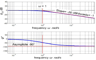
Fig 10.13 Frequency response of a first-order lag in Bode diagram for T = 1. Red straight lines denote high-frequency asymptotes.