nserman@fsb.hr Transfer Function Concept Digest
10. ELEMENTARY BLOCKS
10.1 Static Gain
The elementary block described by (10.1) is presented in fig 10.1 as an autonomous system which is commonly referred to as static gain.
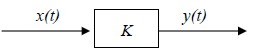
Fig 10.1 Block presentation of static gain
Dependence of the output y(t) on input x(t) is defined in the time domain by a zero-order differential equation which contracts to algebraic equation:
![]()
where K is a constant with dimension: ![]() [brackets denote ‘dimension of’].
[brackets denote ‘dimension of’].
When x and y are relative, i.e. dimensionless variables, K is dimensionless as well. The use of relative variables is assumed throughout the following paragraphs.
Static gain maps input function x(t) into the output y(t) without any dynamical distortion, as it is demonstrated in fig. 10.2 using the step response as an example.
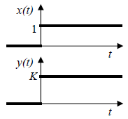
Fig 10.2 Step response of a static gain (unity step at input)
The equation (10.4) is mapped into the frequency domain as the transfer function:
![]()
For s = j ω the transfer function (10.5) defines frequency response presented in Bode diagram in fig. 10.3 and in Nyquist diagram in fig. 10.4.
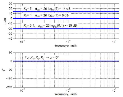
Fig 10.3 Frequency response of a static gain (three different values of K) in Bode diagram
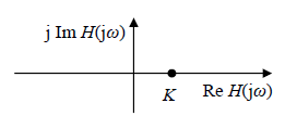
Fig 10.4 Frequency response of a static gain in Nyquist diagram (K is a real number)