Nikola Šerman, prof. emeritus                                                                                  Linear Theory
nserman@fsb.hr                                                                                                         Transfer Function Concept Digest

6. FREQUENCY RESPONSE

Physical meaning

The system defined by the equation (2.1), or by the corresponding transfer function H(s), would respond to any excitation x(t) by a change of the output y(t) that would be a sum of transients y(t)_t and particular solution y(t)_p.

If input signal x(t) changes harmonically, e.g. by a sinus function, a particular solution of equation (2.1) would also be a sinus function at the same frequency as the input.  However, the output y(t) would have a different amplitude as well as a certain phase shift with respect to the input (fig. 6.1).

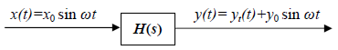
Fig. 6.1 Response of the system H(s) to a harmonic excitation (ω – angular frequency in rad/s)

Providing the subject system is stable, after a certain time period the transients would vanish with only a particular solution to remain.

The response of such an arbitrarily chosen system to a harmonic (sinusoidal) excitation with the initial state of the system being perturbed (non-zero initial condition) is shown in fig. 6.2.  The response itself is a sum of transients y(t)_t and a particular solution y(t)_p.  These two are plotted separately.  The transients practically vanish in about 12s. After that the output y(t) is made solely of a particular solution y(t)_p.

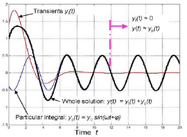
Fig. 6.2 Example of an arbitrary stable system’s response to a harmonic (sinusoidal) excitation (non-zero initial conditions)

Fig. 6.3 shows simultaneous plots of the input and the output.  The ratio of their harmonic changes (after the transients vanished) depends on the input frequency ω.  This ratio is often called dynamic gain:

The phase shift φ also depends on the frequency ω. It can be determined by time-shift Δt (fig 6.3):

If the output follows the input then the phase shift is considered as negative, consequently if it precedes the input the phase shift is positive.

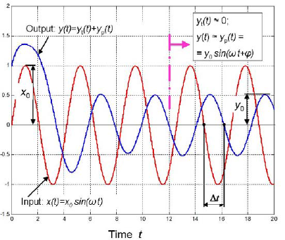
Fig. 6.3 Input and output functions of the system from fig. 6.2

The function from equation 6.1 is often called amplitude-frequency characteristic.  The function is called phase-frequency characteristic.

System Frequency Response In Bode diagram

These both functions can be plotted in Bode diagram.  They are plotted separately in their respective coordinates against common frequency that is logarithmically scaled.

Dynamic gain is usually expressed in decibels [dB] where:

The ordinate of amplitude-frequency characteristic, which represents dynamic gain α_dB, is plotted in a linear scale.  As , the unity distance in the ordinate direction equals 20 dB which denotes a ten-fold increase in dynamic gain..

Some examples of α and α_dB relation are shown in the following table:

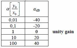
The value of dynamic gain α expressed as a ratio of the amplitudes can be calculated from α_dB by formula α = 10^0.05α_dB.

The phase shift, being the phase-frequency characteristic ordinate, is plotted in a linear scale.  It is expressed either in radians or in degrees.

Frequency characteristics in Bode diagram is shown in fig. 6.4

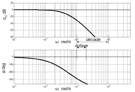
Fig. 6.4 Frequency characteristics of the same system as in fig. 6.2, presented in Bode diagram

Due to the fact that  , the unity distance in frequency logarithmic scale corresponds to a frequency ten-fold increase.  It  is referred to as decade.  The interval of a double frequency is often referred to as octave.

Amplitude-frequency and phase-frequency characteristics together are dynamic system properties. They are usually denoted as the system frequency response.

System Frequency Response In Nyquist diagram

System frequency response can be presented in a parametric form, i.e. by a single function α(φ) in which frequency ω appears as a parameter.  Such a frequency response presentation that is plotted in the polar coordinates is referred to as Nyquist diagram.

Nyquist presentation of the the same frequency response presented by Bode diagram in fig. 6.4 is shown in fig. 6.5.

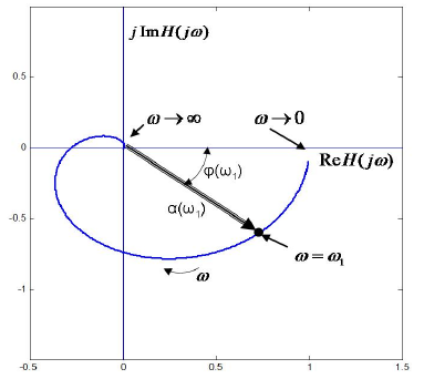
Fig. 6.5 Nyquist diagram presentation of the same frequency response presented by Bode diagram in fig. 6.4

There in fig. 6.5 there are Cartesian coordinates plotted together with the polar ones. Such a combination reveals a very important relationship between the transfer function and the frequency response.

When the real part of complex variable s equals zero, i.e. when s₁ = jω₁, the corresponding point of the transfer function H(s₁)_s=jω1 = H(jω₁) exactly coincides with the frequency response point in Nyquist diagram.

This means that any given linear system transfer function H(jω) presents the system frequency response in Nyquist coordinates:

Therefore the Cartesian coordinates in fig. 6.5 refer to the real and to the imaginary part of the transfer function H(jω) respectively.