10. ELEMENTARY BLOCKS

10.6 Second Order Oscillator

Elementary block named second-order oscillator offers somewhat closer insight into oscillatory transients, as well as into the resonance which often occur in closed-loop systems.

Poles of the transfer function (4.3) are the roots of its denominator which is a polynomial of n-th order.   Depending on the polynomial coefficients there can be some complex roots.   As in physical systems all the coefficients are real numbers so the complex roots always appear in conjugate pairs.  A pair of complex poles of the transfer function (4.3) has a form of  and  .

Transient corresponding to such a pair of complex poles is a damped oscillatory function:

Although the poles Cartesian coordinates σ₀ and ω₀ completely define the shape of the corresponding transient, each of them separately contains very reduced information on the transients shape. It is shown in fig. 10.21.

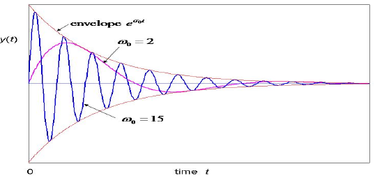
Figure 10.21 Two different transients for the same σ₀, but different ω₀ values.  The envelope is the same, however the damping is completely different.

Much better insight into the oscillator dynamics, including its damping and resonance, is provided by means of the polar coordinates.  Fig. 10.22. shows how natural frequency and damping ratio are defined in the polar coordinates.

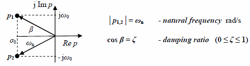
Figure 10.22. Definitions of natural frequency ω_n and damping ratio ζ  by means of polar coordinates of poles in the complex plane

Damping ratio  ζ  provides the information on the transients shape regardless of the frequency.  Natural frequency ω_n determines solely the time scale in which the transient occurs.  This is demonstrated by unity-step responses in fig. 10.23.  Four different damping ratio values responses are plotted against the relative dimensionless time axis.

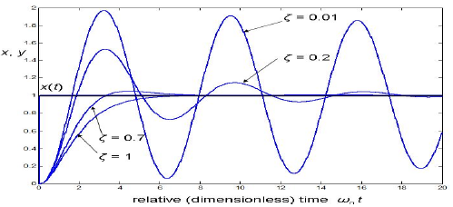
Figure 10.23 Second-order oscillator unity-step responses for four different damping ratio values.  The absolute time scale of abscissa depends on ω_n.

Second-order oscillator transfer function in its original form (10.16) is a special case of (4.3).  However, in this form it gives no idea about the dynamic properties of the block itself.

Therefore it is more convenient to express it in terms of natural frequency ω_n , damping ratio ζ , and static gain K as it is shown in fig 10.24.

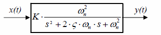
Figure 10.24 Second-order oscillator block presentation expressed in terms of natural frequency ω_n , damping ratio ζ , and static gain K

Relations between natural frequency ω_n , damping ratio ζ , and static gain K on one side, against a₂, a₁, a₀ and C from (10.16)  is given in (10.17):

Frequency response in Bode diagram for three different damping ratio values ζ is presented in fig. 10.25.

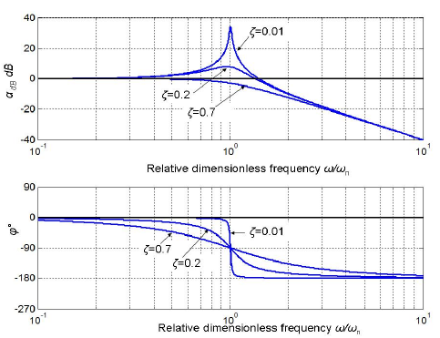
Figure 10.25 Second-order oscillator frequency responses in Bode diagram for three different values of damping  ratio ζ.

The peak in the amplitude-frequency characteristic indicates the resonance.  Its prominence rises with lowering the damping ratio.  The range of ζ as presented in fig 10.25 is 0.7 > ζ > 0.01 .  The  extreme value of dynamic gain is denoted by α_R and named resonance factor.  It rises from 1 to infinity with lowering ζ value.  Interrelation between resonance factor α_R and damping ratio ζ is defined by (10.18).  It is graphical presented in fig. 10.26.

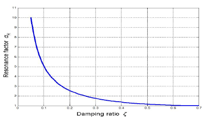
Figure 10.26 Interrelation between resonance factor α_R and damping ratio ζ

The resonance manifests itself when an oscillator is excited by a harmonic input with the frequency close to ω_n.  The resonance factor α_R occurs at the frequency ω_R which is slightly different then the natural frequency ω_n. The difference between these two depends on the damping ratio ζ as it is shown in (10.19).