nserman@fsb.hr Transfer Function Concept Digest
13. LIMITATIONS WITH APPLYING TRANSFER FUNCTION CONCEPT TO REAL-WORLD DYNAMIC SYSTEMS ANALYSIS
Introduction
Notion system as used in the preceding pages is an abstract methodological tool in approaching the causes and effects within some deliberately extracted portion of the universe. System content and its boundaries are defined by the analyst in order to make analyses feasible and useful with respect to a given purpose.
System consists of one or more components connected by interactions and separated from the rest of the universe by boundaries through which system interacts with its surrounding.
Mathematical description of the causes and effects within a system itself as well as between the system and its surrounding is called mathematical model. Same system may be described by a variety of mathematical models, depending on the purpose of a model, relevant variables and required accuracy.
All dynamic systems in real world are nonlinear and with distributed parameters.
Linear vs. nonlinear
Linear systems belong to an abstract category of systems which obey the superposition principle as stated in Chapter 2. There are no linear systems the real world.
Distributed vs. lumped parameters
Distributed parameters systems are those in which the variables describing the state of a system depend not only on time, but also on one or more spatial coordinates. For example, in a process of a metal plate heating the metal plate temperature changes in time. Additionally, its value at any instant of time depends on the position within the plate as well. Mathematical models of distributed parameters systems belong to a category of partial differential equations.
Lumped parameters systems are those in which the variables describing the state of a system depend solely on time. Mathematical models of such systems are ordinary differential equations. The above mentioned heated plate can be considered as a lumped parameters system if the purpose of analysis allows accepting the average temperature of a plate at any instant of time as relevant, thus neglecting the differences between temperatures across the plate.
Linearization
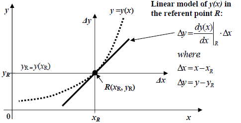
Linear systems concept relies on linearizing nonlinear functions as illustrated in fig. 13.1. Linear model of y(x) is expressed in terms of deviations Δx and Δy:
![]()
Its relation to nonlinear function y(x) is defined by:
![]()
As per (13.2), linearization at a chosen referent point R(xR , yR) is possible if at least the first derivative of y(x) exists at the same point. A nonlinear system linear model is obtained when all the nonlinear functions in its mathematical model are substituted by their linear approximations according to (13.2).

Figure 13.1 Nonlinear function y=y(x) and its linear model obtained by linearization in a referent point R.
When using the transfer function concept prerequisites from the previous chapters it is important to keep in mind the idea of linearization and its effects on trustworthiness of the model itself.
Linear model describes dynamic properties of the nonlinear system in the vicinity of referent point only, i.e. when deviations from this point are small enough. What does “small enough” means in particular case depends on the character of nonlinearities involved and expected accuracy of your analysis.


